möchte­gern­geek

My favorite problems are those which seem simple but exhibit unexpected depth. A prime example is the Traveling Salesperson Problem: It is simple to understand that the garbage truck needs to collect every garbage container, while trying to take the shortest route.

But here, I want to talk about the problem of the longest increasing subsequence (LIS): For a given sequence of numbers, find the subsequence consisting of increasing numbers, which is longest.

This problem is so simple that it was first studied almost as a placeholder by Stanisław Ulam in a book chapter describing the Monte Carlo method. And judging by the google results, it seems to be a common problem posed to university students. I am wondering how many job applicants were distressed when trying to solve it in front of a whiteboard.

However, apparently one can write whole books about this problem. It turns out that there are surprising connections to seemingly independent problems. For example, the length \(L\) of a LIS of a permutation fluctuates the same way as the distance from the center to the border of a coffee stain or the largest eigenvalues of random matrices.

The solution of this problem is not unique: A Sequence can contain multiple longest increasing subsequences. Indeed, their number grows exponentially with the length of the original sequence.

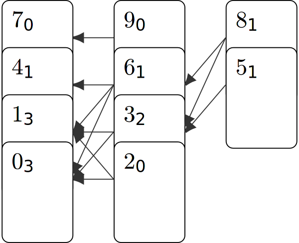
![Different longest increasing subsequences within the same sequence](/img/lis_alternatives.png]{: .invertable}

But up to now, there did not exist any results about the precise number of different LIS. A common sentiment is that counting all LIS was infeasible, since there are exponentially many. And that would be true if we would want to enumerate them. But since we only want to now the number, we can use dynamic programming to determine it efficiently. The basic idea is that we calculate for each element that can appear at position \(x\) in a LIS of how many increasing subsequences of length \(L-x\) it is the first element.

This becomes easy thanks to a datastructure encoding which elements can be subsequent in a LIS. For this we extend Patience Sort. Since the algorithm is called after a game of cards, it is adequate to describe it with cards: We write each element of our sequence on a card and sort the deck according to the sequence such that the first element is on top. Then we take cards from the top of the deck. We put the topmost card on the table opening a stack. We put the next card on the first stack whose top card is larger than it or open a new stack right of the currently rightmost stack. Each time we put a card on the table, we also add pointers to all cards of the stack left of the placed card which are smaller. These are the cards which could be its predecessor in a LIS.

In the end there are \(L\) stacks, where \(L\) is the length of the LIS. We can start from the rightmost stack, select an arbitrary element and follow the pointers to build a LIS. If we were only interested in the length, we could disregard all but the top card of every stack and could simply the algorithm:

fn lis_len<T: Ord>(seq: &[T]) -> usize {
    let mut stacks = Vec::new();
    for i in seq {
        let pos = stacks.binary_search(&i)
            .err()
            .expect("Encountered non-unique element in sequence!");
        if pos == stacks.len() {
            stacks.push(i);
        } else {
            stacks[pos] = i;
        }
    }
    stacks.len()
}

But we want more, therefore we annotate each card of the rightmost stack with the number of increasing subsequences of length \(x=1\) of which they are the first element, which is trivially 1 for each card. Then we continue with the stack left of it and annotate how many increasing subsequences of length 2 start with them. We can calculate this easily by following the pointers backwards and add up the annotations of all predecessor cards. After repeating this and annotating the leftmost stack, we can sum all annotations of the leftmost stack to get the total number of distinct LIS: here \(7\).

About the behavior for longer sequences from different random ensembles we published an article.

In this Article, we introduce an ensemble of the Traveling Salesperson problem (TSP) that can be tuned with a parameter \(\sigma\) from the trivial case of cities equidistant on a circle to the random Euclidean TSP in a plane.

For this ensemble we determine some phase transitions from an “easy” phase to a “not-that-easy” phase using linear programming. For each of these transitions we present structural properties of the optimal solution, which change at these points characteristically. Since the optimal solution is independent of the solution method, those phase transitions are not only relevant for the specific linear program respectively the solver implementation used to solve them, but a fundamental property of this TSP ensemble.

We used the classical linear program of Dantzig:

Here \(c_{ij}\) is the distance matrix between all pairs of cities of \(V\) and \(x_{ij}\) is the adjacency matrix, i.e., \(x_{ij} = 1\), if \(i\) and \(j\) are consecutive in the tour and \(x_{ij} = 0\) otherwise. Therefore, the first line minimizes the length of the tour. To avoid that we conclude that \(x_{ij} = 0\), i.e., staying at home, is identified as the optimal tour, we introduce the third line to force each city to have two connections, enough to enter and leave. But our salesman is clever and can trick us by choosing \(x_{ij} = 0.5\). Since we can not interpret this, we introduce line 2 to force all \(x_{ij}\) to integers. Still valid are two unconnected tours, which we forbid with the fourth line, the subtour elimination constraints. Well, the careful reader might already see that we defined one constraint for each subset of the cities, which are exponentially many in the number of cities. But we can solve this by starting without this class of constraints and only adding the ones which are actually violated by a solution. The violated ones can luckily be found easily by calculating the minimum cut of the proposed solution. The corresponding constraint can be added and the procedure is repeated until no subtour elimination constraint is violated anymore.

So does that mean that we found an efficient algorithm to solve the traveling salesperson problem? No, unfortunately we can not claim the Millenium Prize yet. There is no known algorithm which can efficiently solve this problem under the integer constraint. But if we drop this constraint, we can use efficient algorithms of linear programming to solve the relaxation. The resulting length will always be a lower bound on the actual solution and if we, by chance, find an integer solution, we can be sure that it is actually the optimal solution.

As the order parameter of the transitions from easy to hard we use the probability that a simplex solver yields an integer, and therefore optimal, solution. Without the Subtour Elimination Constraints, the transition occurs at the point at which the optimal solution deviates from the order of the cities on the initial circle. With the Subtour Elimination Constraints the transition coincides with the point at which the optimal tour changes from a zig-zag course to larger meandering arcs. This is measured by the tortuosity

which is maximal at this point. For the tortuosity the tour is divided in \(N\) parts of same-sign-curvature. For each part the ratio of the direct end-to-end distance \(S_i\) to the length along the arc \(L_i\) is summed.

So, we detected continuous phase transitions in the hardness of the problem with linear programming and correlated them with structural changes.